How is lift created?

In my uni years I went to a lot of science conferences; one of the papers that I remember very was about ships propellers and how it can create thrust. A comparison was made with lift on an aerofoil. As the author put it, the lift appears as a pressure difference on the tow faces of the aerofoil. The difference appears because the velocity of air on the upper is larger than that on the lower face. And finally, this velocity difference is because of the upper edge of the aerofoil section is larger and the particles would have to travel faster in a given time.

This is wrong.

First of all lets clarify some ideas:
1. Lift is a force, and in fluid dynamics forces are the results of pressure differential.
2. The concept that the bigger the velocity, the lower the pressure is based on Bernoulli's equation (conservation of energy), but this can be applied only on the same streamline (see post on lines in FD).
3. There is no law or experiment that states that the particles that split at the leading edge must combine at the trailing edge at the same time; actually there is evidence that in order to create lift, the particles on the upper surface reach the trailing edge before those on the lower surface.

The correct explanation is the following.
The shape of the aerofoil creates pressure gradients; for a curved streamline, the pressure will be higher on the convex side. This pressure differential accounts for the force; from the force and pressure the velocity is derived.

From this the conclusion is that aerofoil profile is the most important for the lift; a straight profile can't create lift.

Read More

Open source solutions for computer aided simulations

Introduction

Any engineering problem can be solved with one of the following approaches: analytical, experimental and numerical; from these, numerical analysis is the single most effective tool that can give insight to virtually any level of detail. Numerical analysis is practically a science placed at the intersection of mathematics, computer science and physics.

The most extraordinary aspect of this science is that it takes shape in computer programs that model the real life and can predict the behavior of matter. I won’t go into details of how this modeling is done or how accurate it is. But it is notable that numerical analysis is becoming more and more used in industry and this trend is sustained by the development of IT.

The first FEA and CFD analyses were performed in ’50 on 1 processor computers that had the size of a large storage cabinet; today one can fit up to 32 processors and 512GB of RAM into a normal size computer; this sure sounds impressive, but interesting things are yet to come.

With the development of hardware, the software also evolved extensively; we can say now that the FEA software has matured in the aspect of accuracy, application and ease of use; the CFD software has also reached a high level of detail insight taking advantage of the visualization developments.

Now all this effort comes at a price, sometimes very high; those that invested in research and development of these wonderful tools must be compensated for their work. The research goes in understanding the physics, creating better numerical schemes and creating better algorithms and interfaces.

Fact is, in the last 20 years or so little was done in the first two directions. The physics and numerical schemes are now available at almost no cost; the biggest endeavors were made in computer science: making the code faster, the interface more intuitive, automating more and more actions. This clearly reduces the time spend and permits average engineer to make a simulation for fast results. But the way I see it, this makes room for problems as well: lack of experience personnel, limitations on problem setup and hidden errors in software.

Commercial vs Open-source

Given that all the information needed to create numerical solution is available, many software solutions appeared; some of them are commercial and others are open-source; commercial means you have to pay for the use of the software; but there are other payments requested for the use of multiple processors, for customer support and training; you cannot use the full computing power until you pay for a license for parallel computing; basically you have pay for everything, and even to use what is yours already.

Open-source on the other hand do not charge for license and let you use all your computing power at no costs; on the other hand they give support and training on demand based on a fee; the fees are comparable with those for the commercial software. Therefore open-source doesn’t mean free as in cost-free, but it can be seen more as the freedom to access the knowledge and resources. The open-source software allows user to access and improve the source code in order to make custom applications.

The open-source community is very active and it is interested in many fields, including engineering; just to see some of the available open-source solutions, I have made a list below:

SOFTWARE	USED FOR
QCAD	2D & 3D CAD
FreeCAD	2D & 3D CAD
SagCad	2D & 3D CAD
Salome	3D CAD Meshing Post Processing
GMSH	Geometry Modelling Meshing Post Processing
enGrid	CFD Oriented Mesher
Discretizer	Structured mesh generator for OpenFOAM
Code Aster	Multiphysics FEA
Elmer	Multiphysics FE package
Impact	Explicit FE Dynamics
Calculix	Pre-post & FE solver, Abaqus-like syntax
MBDyn	Multibody Dynamics
Dynela	Non-linear Explicit Dynamics
Fenics	General purpose FE solver for multiphysics applications
OpenFOAM	Multipurpose CFD Solvers
Code Saturne	3D CFD solver
Gerris	2D / 3D  CFD Solvers
Paraview	General Purpose 3D Visualization
Python	Programming language used for scientific computing
R	Mathematical modelling & statistics (similar to S-Plus)
Scilab	Matlab/Simulink-like mathematical programming environment
Octave	MATLAB compatible mathematical programming
wxMaxima	Maple like symbolic computing environment

Each code has its ups and downs and here is not the place to go into detail and describe how good is each of them and if it could give the same efficiency as the commercial alternative.

A case study on CFD tools

From the beginning I want to be noted that I do not favor any CAE provider, commercial of open. But I think that for the sake of good business, an objective comparison for the ups and downs is appropriate. Therefore, I will compare two alternatives in the field I am more comfortable with.

Let’s take the case of CFD; based on the cfd-online.com software user forums, we have the following usage of solvers (no. of CFD solvers threads on cfd-online forums @ 22.05.2015): 

SOFTWARE	THREADS	% of USERS
FLUENT	41 845	42%
OPENFOAM	29 104	29%
CFX	16 468	17%
CD-adapco	7 595	8%
OTHER	4 305	4%

These data show that the second most used CFD code is OpenFOAM, an open-source code; of course, these figures are subject to discussion. I already mentioned the costs implied; from my opinion, if costs are the most important, OpenFOAM is way cheaper than Fluent.

Another big issue is the accuracy these tools may provide; on the other hand I am obliged to ask what the accuracy of a commercial code is and who grants that? In order to answer this and not favor any party, I will show you the results of Aku Karvinen and Hannu Ahlstedt documented in their paper. Aku and Hannu studied a separated flow in a three-dimensional diffuser using OpenFOAM and Fluent; simulations were performed using two turbulence models in both codes; the setup problem is shown below:

Geometry, dimensions and coordinate systems of the three-dimensional diffuser

A diffuser is a popular separated flow test because of its apparently simple geometry. Many experimental studies have been performed on diffusers and data is available for comparison with numerical results. The working fluid is water that enters the domain with a velocity of 1 m/s; based on the fluid properties and domain dimensions, the Reynolds number is about 10000. 

The objective is to see how well are the velocity components computed with OpenFOAM and Fluent; instances of the velocity distribution are determined at each 3 cm for the first 15 cm of the diffuser. Below we can see a comparison between experimental, Fluent and OpenFOAM results of the x component velocity; two turbulence models have been taken into consideration.

In the following plots one can see the mean streamwise velocities, x component at diffuser cross-sections various distances from the origin using k-ε model; contour lines are spaced 0.1 apart; the zero velocity contour line is thicker than others:

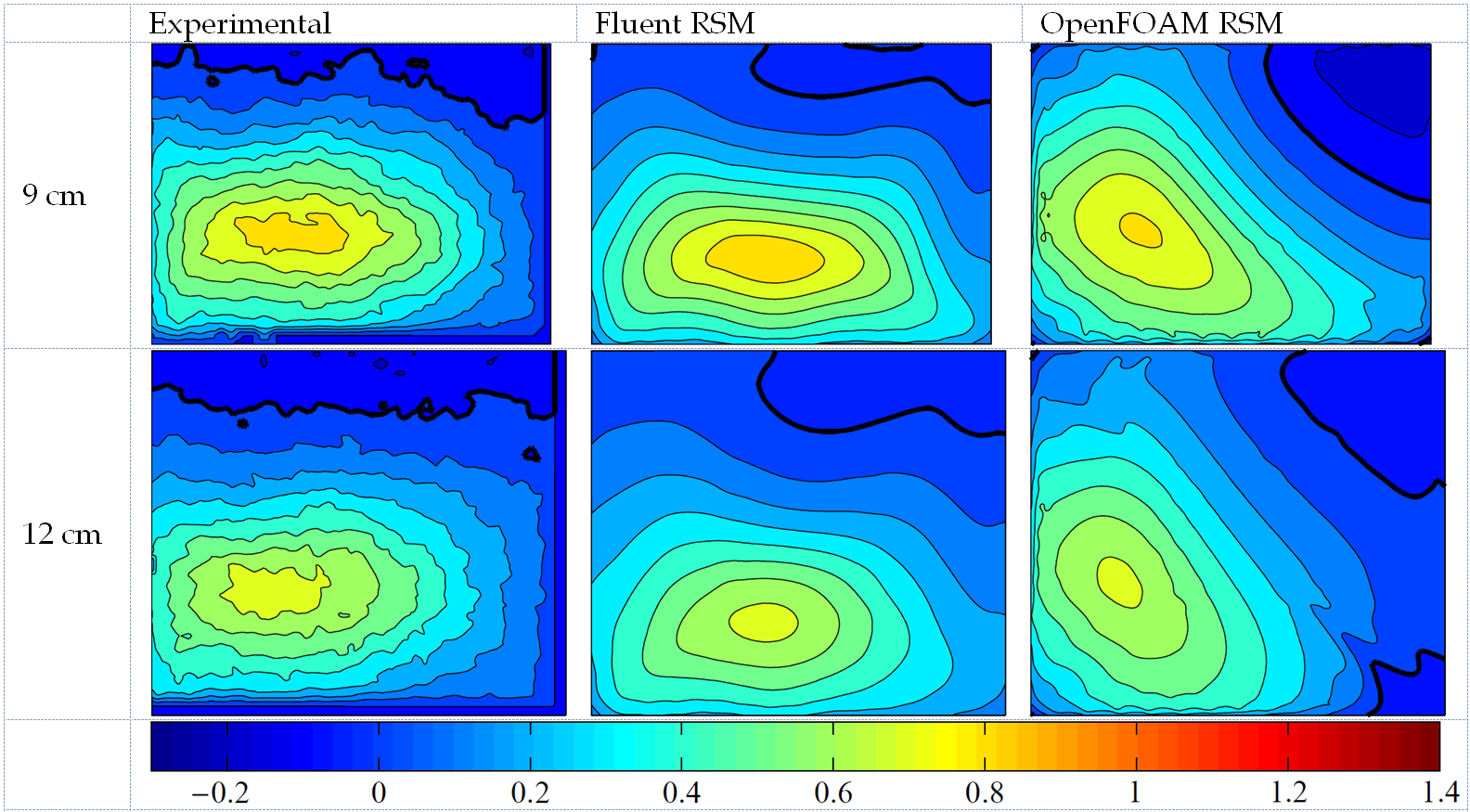
In the following plots one can see the mean streamwise velocities, x component at diffuser cross-sections various distances from the origin using Reynolds Stress model; contour lines are spaced 0.1 apart; the zero velocity contour line is thicker than others:

For even more results, please refer to the original paper; the conclusion that we can get out of the presented plots is that there are considerable differences between results obtained using different turbulence models; the best results are obtained with Reynolds stress model used in Fluent.

Unfortunately this model is rarely used in industrial simulations because it is very time consuming and turbulence models like k-ε and k-ω are faster. Comparing the plots from Fig.2, in which the k-ε was used, one can see very similar results for both codes. Therefore it can be concluded that for the applications used in industry, Fluent and OpenFOAM can give remarkably similar results.

Conclusion

Keep in mind that the success of one open-source solution doesn’t prove that all solutions are good or immediately applicable; but, for the sake of business development I think we can give them a chance to prove their capability.

In this article I showed only a small fraction of what the open-source tools are capable of; in the next issues of the magazine we will go into much greater detail on the opportunities that open-source have to offer.

References:

http://caelinux.com/CMS/

http://www.cfd-online.com/Forums/

Aku Karvinen and Hannu Ahlstedt, Comparison of turbulence models in case of three-dimensional diffuser, available online, at link

Read More

2D Transport of a Passive Scalar with OpenFOAM

All the posts that have been written until now tackled the shockTube problem and the 1D transport problem; we've seen the convection and diffusion at work and we saw that there are a lot different schemes for divergences modelling.
In the following I will show the setup and results for 2D scalar transport problem. This was actually the first problem that I setup and solved from scratch on my own in OpenFOAM.
This may not be a physical problem but it has all the components of an actual CFD problem solved in OpenFOAM.

Problem statement:
- a 2D domain in a shape of a square with the side of 10 m;
- in the middle of the square we have a circle of radius 1 m;

Read More